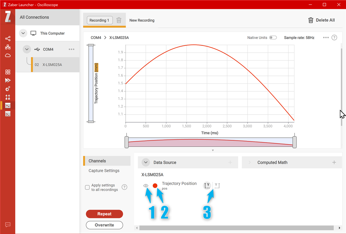
This section covers the basic features of the Oscilloscope application, and its two most commonly used capture modes, polled and buffered.

The video below introduces the main areas of the user interface and shows how to capture and explore data in the two modes.

This video introduces the two main modes of the Oscilloscope, polled (free-running) and buffered (firmware-mediated). It shows how to add additional channels to record, how to start and stop recording, and how to visually explore the recorded data once it is available.

Let's elaborate on some of the less-commonly used controls that are not described in the video. Refer to the blue numbers in the following screenshots.

The visibility eyecon (1) toggles whether or not the corresponding data is shown in the chart.

The color swatch (2) lets you change the displayed color of that data trace. This can also be changed before recording the data, or in the dialog where new traces are added.

The Y axis buttons (3) control whether the trace is grouped on the left or right Y axis of the chart. Grouping traces with similar scales together gives you better visibility of small changes.

The display contains one chart for each collection of traces that have units of measure in the same dimension. That is, if relevant there wiill be a chart for positions, a chart for velocities, another for accelerations etc. If there is more than one chart, scroll down to see the others.

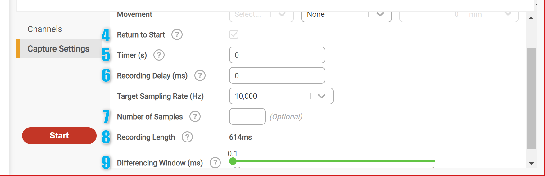
The above screenshot shows controls visible in the Capture Settings panel before starting a recording. Not all of these controls are visible in all modes.

The Return to Start checkbox (4) controls whether the application will return the selected device to its original position once data recording is finished. This applies to both relative and absolute moves. It's recommended to enable this if you want to repeat the same experiment multiple times, as otherwise an absolute move will only physically move the device the first time, and a relative move will eventually hit the end of travel.

The Timer (5) adds a delay between pressing the Start button and actually starting recording. This is used if your experiment is sensitive to table vibration and you need a few seconds to move away after pressing the Start button. This timer is software-controlled.

Recording Delay (6) is a firmware-controlled timer that starts when data capture starts (from the software perspective) but data recording does not actually begin until it expires. This is used to provide more precisely timed recording of a small section of a device movement.

Number of Samples (7) optionally lets you limit how many data samples will be recorded. If you can predict how many samples you need, this may speed up the recording process.

Recording Length (8) is not an interactive control, but shows you a prediction of how much time data can be recorded over given the current setup.

Finally, Differencing Window (9) controls how displayed data is interpolated when the sampling rate is low or irregular. This only affects the calculation of math channels, which uses central differencing as a way to smooth out noise and sampling irregularity. This controls how wide the central differencing window is in time. Making it larger will smooth out noisy calculated traces.